Search Engine using Tf-Idf

Result Consists of Title, Overview, Release Date, Idf Score, Tf Score, Tf-Idf Score for each term and total

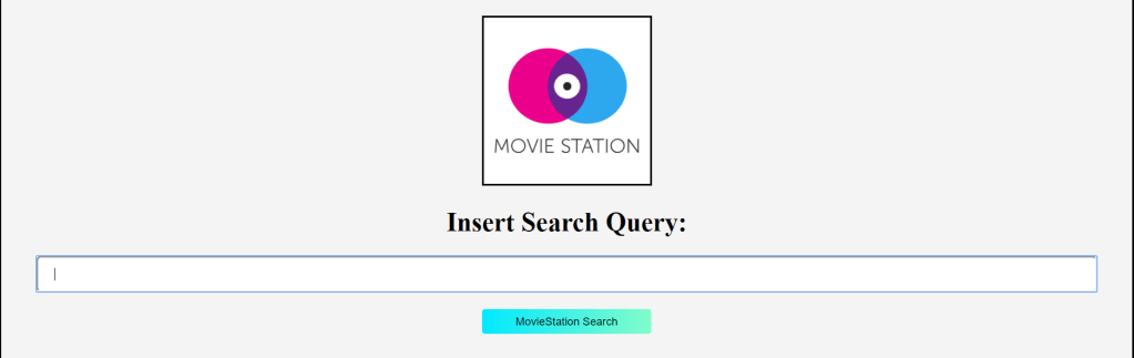
Search Engine plays a very important part of our everyday life. For every small information, we tend to search it on the search engine. So, here is the search engine for the Movie Search using MovieLens Dataset.
The dataset I used is from Kaggle. The dataset consists of Movie data like Movie Overview, IMDB Rating, Release Date, Title, etc.

Data Preprocessing:

So as to make a text search module, first we have to have the fitting dataset that we expect to deal with. On acquiring the informational collection, the dataset must be handled and brought to a comprehensible structure.
Preprocessing of data on a big dataset is an errand, particularly when it contains records of more than 40k. In the dataset that I have utilized, there are movie records with data of multiple movies with its overview, release date, title, etc.
Text Search will be performed on the overview and tagline segment of the dataset, which contains a long length of words. These words are isolated from the string with the assistance of Python’s split function.
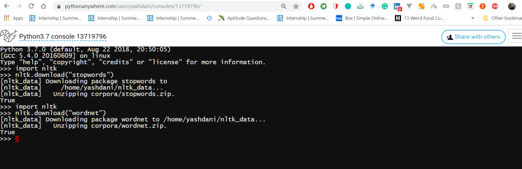
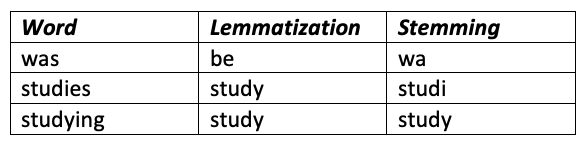
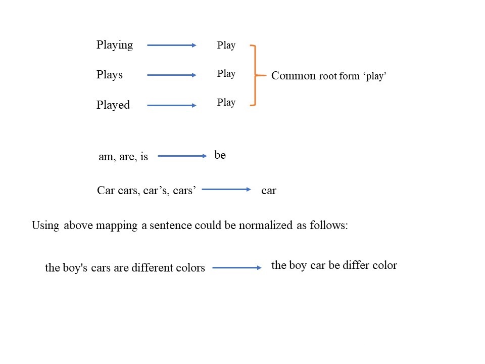
So as to make the pursuit increasingly summed up, the sum total of what characters have been changed over into lowercase letters. After that, I have utilized the NLTK library, which is likely one of the most helpful libraries for normal language processing in Python. We import the stopwords function from the corpus of the module. We can use this to take out the stopwords that are available in the input data. On finishing this, we utilize the lemmatizer function so as to distinguish the base of the words, widening the range for the text-search.

Stemming vs Lemmatization

Creating the Index:

We have to create the inverted index for the dataset then process the queries and show search results:

Inverted Index:
An inverted index is an index data structure storing a mapping from content, such as words or numbers, to its locations in a document or a set of documents.

Tf-Idf:
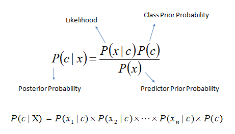
TF-IDF, which stands for term frequency-inverse document frequency, is a scoring measure widely used in information retrieval (IR) or summarization. TF-IDF is intended to reflect how relevant a term is in a given document.

Tf(Term Frequency):
Term Frequency, which measures how frequently a term occurs in a document. Since every document is different in length, it is possible that a term would appear much more time in long documents than shorter ones.
TF(t) = (Number of times term t appears in a document) / (Total number of terms in the document)

Idf(Inverse Document Frequency)
Inverse Document Frequency, which measures how important a term is. While computing TF, all terms are considered equally important. However, it is known that certain terms, such as “is”, “of”, and “that”, may appear a lot of times but have little importance.
IDF(t) = log_e(Total number of documents / Number of documents with term t in it)

Remaining Steps:

  • After creating inverted index, we will build a document vector to calculate the Tf-Idf scores.
  • Then build pickle files using the inverted index and document vector to get the search results for a given input quickly.
  • Then we will calculate the Tf-Idf score for the input given by the user.
  • After this we will calculate it for each term, entered in a input query.
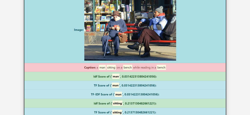
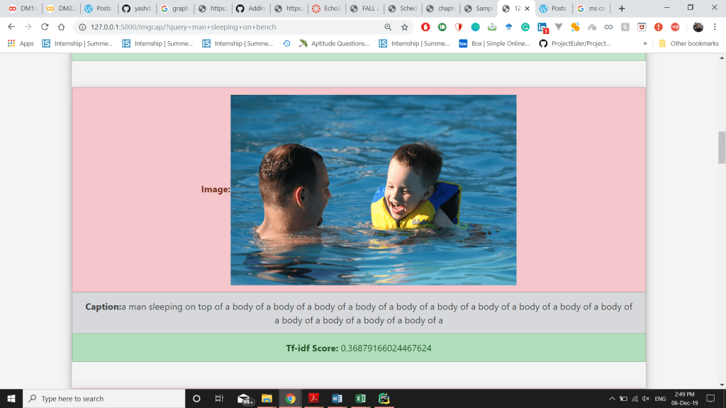
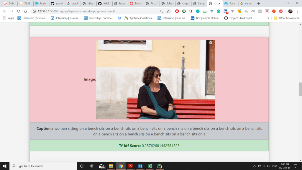
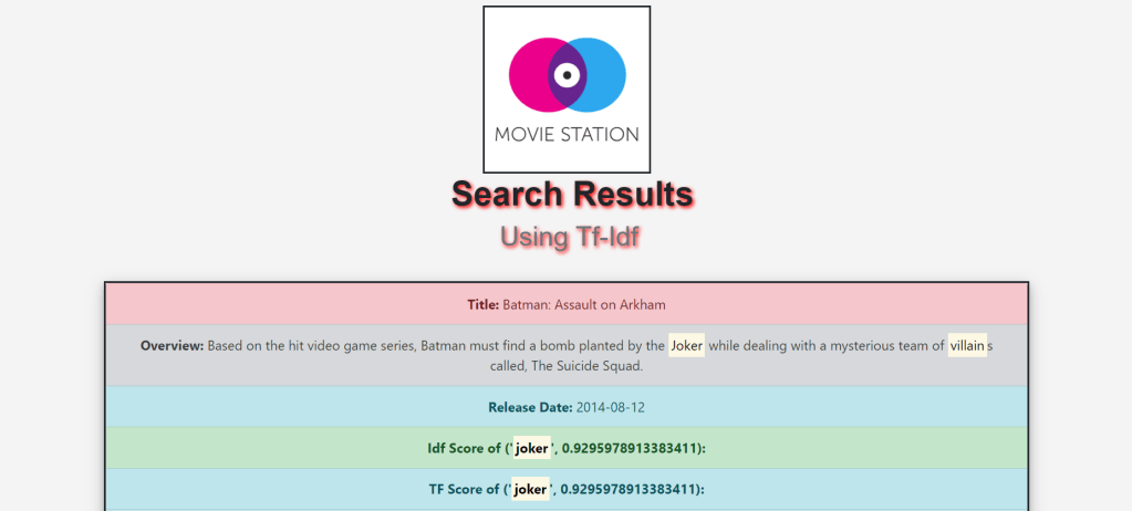
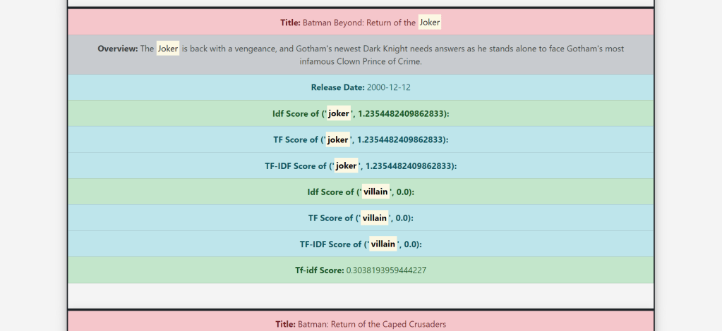
  • And Finally display Tf score, Idf Score, Tf-Idf score,Release date, Overview and Title on the frontend.

Contribution:

  • Use of NLTK’s WordNetLemmatizer
  • Use of NLTK’s stopwords to reduce the unused terms
  • Building Inverted Index
  • Initially, the search time was really high and each search was taking a lot of time due to calculating again and again, so I used .pkl file to store probabilities to save time.
  • Calculating and displaying the Tf-Idf of each input term separately
  • Highlighting the input string on the Web page
One of the contributions – Lemmatization and Stemming
# Created Inverted Index and Document vector along with Tf-Idf Calculations 
def create_inverted_index(self):
        for row in self.meta_data.itertuples():
            index = getattr(row, 'Index')
            data = []
            for col in self.meta_cols.keys():
                if col != "id":
                    col_values = getattr(row, col)
                    parameters = self.meta_cols[col]
                    if parameters is None:
                        data.append(col_values if isinstance(col_values, str) else "")
                    else:
                        col_values = ast.literal_eval(col_values if isinstance(col_values, str) else '[]')
                        if type(col_values) == bool:
                            continue
                        else:
                            for col_value in col_values:
                                for param in parameters:
                                    data.append(col_value[param])
                self.insert(index, self.pre_processing(' '.join(data)))

    def build_doc_vector(self):
        for token_key in self.inverted_index:
            token_values = self.inverted_index[token_key]
            idf = math.log10(self.N / token_values["df"])
            for doc_key in token_values:
                if doc_key != "df":
                    tf_idf = (1 + math.log10(token_values[doc_key])) * idf
                    if doc_key not in self.document_vector:
                        self.document_vector[doc_key] = {token_key: tf_idf, "_sum_": math.pow(tf_idf, 2)}
                    else:
                        self.document_vector[doc_key][token_key] = tf_idf
                        self.document_vector[doc_key]["_sum_"] += math.pow(tf_idf, 2)

        for doc in self.document_vector:
            tf_idf_vector = self.document_vector[doc]
            normalize = math.sqrt(tf_idf_vector["_sum_"])
            for tf_idf_key in tf_idf_vector:
                tf_idf_vector[tf_idf_key] /= normalize

    def build_query_vector(self, processed_query):
        query_vector = {}
        tf_vector = {}
        idf_vector = {}
        sum = 0
        for token in processed_query:
            if token in self.inverted_index:
                # tf_idf = (1 + math.log10(processed_query.count(token))) * math.log10(N/inverted_index[token]["df"])
                tf = (1 + math.log10(processed_query.count(token)))
                tf_vector[token] = tf
                idf = (math.log10(self.N / self.inverted_index[token]["df"]))
                idf_vector[token] = idf
                tf_idf = tf * idf
                query_vector[token] = tf_idf
                sum += math.pow(tf_idf, 2)
        sum = math.sqrt(sum)
        for token in query_vector:
            query_vector[token] /= sum
        return query_vector, idf_vector, tf_vector

Experiments:

  • Ran the code without storing the inverted index and document vector, so it was taking about 3-4 minutes for displaying the search results after all the calculations, this time was saved by using .pkl(pickle file).
  • Ran the code with applying lemmatization before the stemmer, it gave me really good results which were different from when I applied stemmer before lemmatization. Due to this I was able to remove baseword error.
  • Tried to get results without stemming, lemmatization and stopwords removal, it was very different from the desired results and inaccurate.
  • Ran the code using multiple stemmers that is Porter Stemmer, Lancaster stemmer and snowball stemmer and checked the results generated by each of them.
  • Tried to implement synonyms feature using NLTK wordnet in my system on localhost, the implementation was not very accurate due to which I was getting completely irrelevant results.
  • I tried running the code without Idf normalization (Logarithm of Idf score), due to which I was getting very high Tf-Idf score of all the terms and results, with normalization, I got accurate results with the relevant Tf-Idf scores.
# use of lemmatizer, Stemmer, Stopwords and Tokenizer   
 def __init__(self):
        # Data Fetch
        # data_folder = 'C:/Users/yashd/PycharmProjects/txt_search/'
        self.meta_cols = {"id": None, "original_title": None, "overview": None, "release_date": None}
        meta_data = pd.read_csv('movies_metadata.csv', usecols=self.meta_cols.keys(), index_col="id")
        self.meta_data = meta_data.dropna(subset=["overview"])
        self.N = self.meta_data.shape[0]

        # Pre-processing
        self.tokenizer = RegexpTokenizer(r'[a-zA-Z0-9]+')
        self.stopword = stopwords.words('english')
        self.stemmer = PorterStemmer()
        self.lemmatizer = WordNetLemmatizer()
        
        self.inverted_index = {}
        self.document_vector = {}

        if os.path.isfile("invertedIndexPickle.pkl"):
            self.inverted_index = pickle.load(open('invertedIndexPickle.pkl', 'rb'))
            self.document_vector = pickle.load(open('documentVectorPickle.pkl', 'rb'))
        else:
            print("In else of get_scores:")
            self.build()
            self.save()

Challenges Faced:

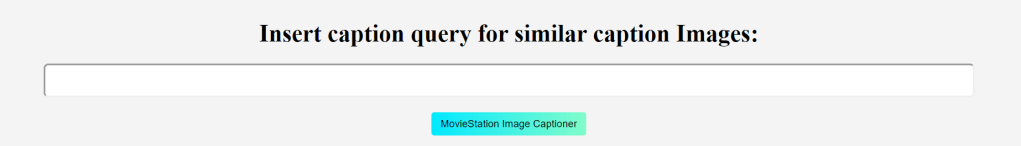
  • Deployment on the web, using python Flask. To solve this issue, I read a lot about it from multiple sources also asked people who knew about it.
  • Hosting the site on Pythonanywhere, for this also I read the documentation along with some other sources to solve the issue.
  • Initially, the search time was really high and each search was taking a lot of time due to calculating again and again, so I used .pkl file to store probabilities to save time.
  • Calculating the Tf-Idf of each term separately
  • Highlighting the input string on the Web page
  • An issue with the NLTK import in pythonanywhere.
# To get the final score
    def get_movie_info(self, sorted_score_list, tf_new, idf_new, tf_idf_new):
        result = []
        for entry in sorted_score_list:
            doc_id = entry[0]
            row = self.meta_data.loc[doc_id]
            info = (row["original_title"],
                    row["overview"] if isinstance(row["overview"], str) else "", entry[1], idf_new[doc_id],
                    tf_new[doc_id], tf_idf_new[doc_id], row["release_date"])
            result.append(info)
        new_score = None
        # print(result[0:5])
        return result

References:

Image Search and Caption Generation

Image Captioning is the process of generating a textual description of an image. It uses both Natural Language Processing and Computer Vision to generate the captions.

In this project, I have implemented an image search feature. For the search feature, first, we have to generate a caption for the images present in our database. For caption generation, we will go through the TensorFlow tutorial. Then we will apply TF-IDF indexing over the captions and implement the search feature. The dataset used for the image captioning model is the MS-COCO Dataset, which is a dataset of images easily accessible by everyone.

Data Preprocessing

The Flickr 30K data set contains 30,000 images. I took 2000 images from these 30,000 images of the Flickr 30K dataset. These 2,000 images have been uploaded to this repository serving as a file server.

Steps to train the Model:

  • Download and extract MS-COCO dataset
  • Store captions and image names in vectors, and select first 30,000 captions from it along with its corresponding images to train our model.
  • Use InceptionV3 pretrained (on Imagenet) to classify each image and extract features
  • Initialize InceptionV3 and load the pre-trained Imagenet weights. After this, create a tf.keras model where the output layer is the last convolutional layer in the InceptionV3 architecture.
  • For Pre-processing, tokenize the captions and pre-process each image with InceptionV3 and cache the output to disk. Caching the output in RAM would require higher memory space but it would be faster, and the required floats per image would be 8 * 8 * 2048.
  • By tokenizing the captions, we will obtain a vocabulary of all the unique words in the data.
  • After that, we will limit the vocabulary size to 5000, to save memory. Then, we’ll replace all other words with the token “UNK” unknown. And then create word-to-index and index-to-word mapping.
  • Since, we have already extracted the features from the lower convolutional layer of InceptionV3 giving us a vector of shape (8, 8, 2048). So, we squash that to the shape of (64, 2048).
  • This vector is then passed through the CNN Encoder. And then, the GRU attends over the image to predict the next word.
  • Now, use the teacher forcing to decide the next input to the decoder, and then finally calculate the gradients and apply it to the optimizer and backpropagate.
  • So basically, after training the model, a CSV file was opened, and, with the help of a for loop, the testing part of the model was made to run for the number of iterations that were equal to the number of images that were being tested.
  • Then the caption, along with the URL of the image was recorded in a .csv file and the captions were tokenized after that calculate the TF-IDF scores of the predicted caption and display the top-10 results along with the image.

Code to iterate from each image and make .csv file for image and generated caption:

import csv

headers = [['id', 'url', 'caption']]
with open('caption_img.csv', 'w') as csvFile:
  writer = csv.writer(csvFile)
  writer.writerows(headers)
csvFile.close()
import csv

with open('caption_img.csv', 'a') as csvFile:
  writer = csv.writer(csvFile)
  for i in range(200,2151):
    image_url = 'https://raw.githubusercontent.com/yashdani/ImgCap/master/' + str(i) + '.jpg'
    image_extension = image_url[-4:]
    image_path = tf.keras.utils.get_file('new_' + str(i) + image_extension, origin=image_url)

    result, attention_plot = evaluate(image_path)
    caption = ' '.join(result)
    print(caption)
    writer.writerows([[str(i), image_url, caption]])
csvFile.close()
print('csv created')

Contributions:

  • Wrote the code for creating .csv file, for taking in a large number of images and storing the created captions in a .csv file.
  • Built the dataset with around 2,000 images from the Flickr dataset and then predicted the captions for those images.
  • Initially, the search time was really high and each search was taking a lot of time due to calculating again and again, so I used .pkl(pickle) file to save search time.
  • Revamped the code of my text search to do the caption search along with images.
  • Uploaded images onto a GitHub repository, which made access to the image URL much easier.

Experiments:

  • Used the Flickr dataset’s CSV file which already had very accurate captions of the images then I trained the model and ran all the images on the model to generate caption, the caption generated for the same images was very different for the captions in the original csv of flickr dataset.
  • Tried to store images at multiple cloud platforms to fetch and display on the frontend, and finally settled on the github to store all my images and fetch to get the desired results.

Challenges Faced:

  • Training of the model took a lot of time, around 3-4 hours. Even on the Google Colab notebook.
  • The use of Google Colab was itself was a difficult task for the people using it for the first time.
  • The timeout of server connections lead to incomplete training of the model, and had to be restarted from the first. This issue was resolved by using an extension in chrome working as a replacement to a mouse click.
  • Difficulty in creating the dataset using only the images. Extracting all the images with the caption in a .csv file using colab was difficult.
  • Understanding the concepts of Neural networks and Deep Learning in a short period of time.
Images with wrong Caption
Images with correct Caption but repeated multiple times

References:

Text Classification by Naive Bayes Classifier

Classification is a process related to categorization, the process in which ideas and objects are recognized, differentiated and understood. Classification task is the process of predicting a class when multiple data points are given. This classifier uses a training data to understand how the variables that are given as input, identify with a specific class.  Out of multiple classification algorithms, Naive Bayes is the one I am using for this project as it gives better performance than others.

In this project, I implemented a text classifier to classify movie genres according to the input given by the user. The dataset consists of many movies with multiple genres so it is a multi-class classification. Text classification helps identify the classes based on the multiple columns data(Overview, etc.).

Naive Bayes Classifier

The Naive Bayesian classifier is based on Bayes’ theorem with the independence assumptions between predictors. A Naive Bayesian model is easy to build, with no complicated iterative parameter estimation which makes it particularly useful for very large datasets. The classification is carried out by calculating the probability of each given class, and displaying the classes with the highest probabilities as the output.

Bayes theorem provides a way of calculating the posterior probability, P(c|x), from P(c), P(x), and P(x|c). Naive Bayes classifier assume that the effect of the value of a predictor (x) on a given class (c) is independent of the values of other predictors. This assumption is called class conditional independence.

  • P(c|x) is the posterior probability of class (target) given predictor (attribute). 
  • P(c) is the prior probability of class
  • P(x|c) is the likelihood which is the probability of predictor given class
  • P(x) is the prior probability of predictor.

t1, t2, t3, … = Terms in data

Formula Used:

Probability(Genre|[Term1, Term2, Term3, …, Termn]) = Probability(Genre) * Probability(Term1|Genre) * Probability(Term2|Genre) * Probability(Term3|Genre) * … * Probability(Termn|Genre)

Procedure:

In the given movielens dataset that has been downloaded from Kaggle, the column that has the genres of the movies is going to be predicted with the help of a given overview or plot of the movies.

For the evaluation step, the data can be divided into training data, testing data. In the given dataset, the training and testing data is divided into 80% and 20% respectively. The dataset has 45,467 records. So, it is divided as 36,374 records for training data and 9,093 records for test data.

Now using Naive bayes algorithm,

  • we find out the prior probability P(c) and P(x)[Formula given above]. Number of records in class c divided by total number of records.
  • Then we find out the conditional probability, by calculating the frequency of a term in a record, of class x or c. P(x|c) and P(c|x).

After this whenever their is input for the classification, we do the preprocessing and filtering of the collection using stemming, lemmatization and removal of stopwords.

After evaluation, a score will be given to each class and using this score the genre is predicted according to the input query.

Now, to calculate the Accuracy, we send the movie overview(plot) of the test data to the input of the training data and then compare the predicted and actual genres of that movie overview.

My Contributions:

  • The model was working on the whole dataset. So, splitting the dataset into test data and train data was done by me. Along with training it to get results along with the accuracy.
  • The classification time to predict the genre was taking alot of time due to calculating again and again, so I used .pkl file to store probabilities to save time.
  • Since the model was not trained, there was no evaluation metrics. I calculated the accuracy of the model as my evaluation metrics.
  • Display the data in the charts to show the result in better orderly manner and also so that the user can see the predictions clearly. And how much is the percentage of each Genre.
  • The classifier was built from scratch to implement the Naive bayes classification, without using any library.
# Code to save probabilities in pickle files
def get_results(query):
    global prior_probability, post_probability
    initialize()
    if os.path.isfile("classifierPicklePrior.pkl"):
        prior_probability = pickle.load(open('classifierPicklePrior.pkl', 'rb'))
        post_probability = pickle.load(open('classifierPicklePost.pkl', 'rb'))
    else:
        (prior_probability, post_probability) = build_and_save()
    return eval_result(query)

Experiments:

  • I also implemented the SVM(Support Vector Machine) using the Skearn library because of that I was able to changes in the Accuracy, it went up to 58.39% using that.
  • For the Naive Bayes classifier, I used multiple ratios for the training and testing data split like 70:30, 80:20, 90:10 etc. respectively and I was able to see the difference in the accuracy of percentage between 37%-45%. Initially, I was comparing the results from one of the genres of the overview input, but when I tried it for comparision with the multiple genres I got the accuracy of 57.44%.
# Code to calculate Probabilities from the tokens
    for (genre, token) in token_genre_count_map:
        post_probability[(genre, token)] = token_genre_count_map[(genre, token)] / token_count

    prior_probability = {x: genre_count_map[x]/row_count for x in genre_count_map}
    save(prior_probability, post_probability)
    return (prior_probability, post_probability)
#Code to show final results
def eval_result(query):
    processed_query = pre_processing(query)
    sum=0
    genre_score = {}
    perc = []
    notrequiredlist={'Vision View Entertainment', 'Aniplex', 'GoHands', 'BROSTA TV', 'Rogue State','Carousel Productions', 'Odyssey Media', 'Sentai Filmworks', 'Pulser Productions', 'Mardock Scramble Production Committee', 'Telescene Film Group Productions', 'The Cartel' }
    for genre in prior_probability.keys():
        if genre in notrequiredlist:
            continue
        score = prior_probability[genre]
        for token in processed_query:
            if (genre, token) in post_probability.keys():
                score = score * post_probability[(genre, token)]
        genre_score[genre] = score
    sorted_score_map = sorted(genre_score.items(), key=operator.itemgetter(1), reverse=True)
    # sorted_score_map = sorted_score_map*10000000
    # print(sorted_score_map)
    for i in sorted_score_map:
        sum += i[1]
    for i in range(len(sorted_score_map)):
        perc.append([sorted_score_map[i][0], sorted_score_map[i][1], (sorted_score_map[i][1] / sum) * 100])
    return perc, sorted_score_map
# Code to check Accuracy
def testAccuracy(test_data):
    num_correct_predictions = 0
    print(type(test_data), test_data)
    for index in list(test_data.index):
        y_result = test_data.at[index, 'genres']
        query = test_data.at[index, 'overview']
        y_predict = get_results(query)[:5]
        for genre in y_predict:
            if y_result == genre[0]:
                num_correct_predictions+=1
    accuracy = num_correct_predictions/len(test_data)
    return accuracy

Challenges Faced:

  • The accuracy got is 39.6% for a split estimation of 0.3 The reason behind why the accuracy is so low is a direct result of the blemish in the language that has been utilized in the dataset, and furthermore, as a wide assortment of words have been repeated in a different classes. So, when I changed the split ratio to 80:20, with removing some of the unwanted genres I got the accuracy of 42.63%.
  • The classification time to predict the genre was taking alot of time due to calculating again and again, so I used .pkl file to store probabilities to save time.
  • Due to lack of Machine Learning Knowledge, the conceptual understanding of Machine Learning Classifier was not clear and it took me lot of time on that along with the issues of training a model. It took me alot of time to fully implement the concept.

References:


Design a site like this with WordPress.com
Get started